Free tools Windows power users keep installed
One-click scans. No signup required.
Crashes, No Sound, or Screen Glitches?
Random freezes, missing sound and display glitches usually trace back to one bad driver. Find and replace yours safely.Free scan · under a minutePC Slower Than It Used to Be?
A free scan shows the junk files, broken settings and background clutter dragging Windows down - then fixes them in one click.Free scan · Windows 10 & 11ThatPainter is reader-supported. When you buy through links on our site, we may earn an affiliate commission. Learn More
You can turn an ordinary Excel grid into a Christmas tree with changing lights using three standard features: cells as pixels, RANDBETWEEN (or RAND) for random light values, and conditional formatting for the colors. Press F9 and Excel recalculates the formulas, producing a new light pattern. It is not an official Christmas Easter egg—just a clever use of tools Excel already has.

As an Amazon Associate I earn from qualifying purchases.
What makes the tree “twinkle”
The effect has three layers:
- The drawing: narrow columns and short rows become square pixels. Green-filled cells form the tree, with separate cells for a trunk and star.
- The light selector: each light cell contains a volatile random formula.
=RANDBETWEEN(1,3)returns 1, 2, or 3 and generates a new value when Excel recalculates. - The color engine: conditional formatting translates those values into colored icons or fills.
Because RAND and RANDBETWEEN recalculate, pressing F9 changes the values and therefore the visible lights. That is manual, recalculation-driven animation—not a continuous timer.
Microsoft documents conditional-formatting rules, icon sets, formula-based rules, rule order, and the Show Icon Only option in its conditional-formatting guide.
#1 Best Overall
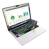
- Microsoft Excel keyboard cover with over 60 color-coded shortcuts for spreadsheets, analysis and finance work, printed over each key.
- Work faster in Excel for Mac: quickly find navigation, formatting, formula and selection commands to reduce repetitive mouse clicks.
- 0.3 mm ultra-thin silicone keyboard protector keeps fast spreadsheet keystrokes responsive while common Excel shortcuts stay in view.
- Washable protection helps keep dust, crumbs and everyday spills off the keyboard. Remove, rinse, dry and reuse. Includes a 12-month warranty.
- Fits MacBook Pro 14/16 (M1-M5), MacBook Air 13/15 (M2-M5) and MacBook Neo 13 (A18 Pro). US English ANSI layout.
Build the basic tree (no VBA required)
1. Make a pixel-art canvas
- Open a blank workbook.
- Select a modest block of cells, such as columns B through N and rows 2 through 20.
- Reduce column width and row height until cells look approximately square. Exact dimensions vary by font and Excel edition.
- Fill cells in widening rows to create a triangular tree. Use green for the foliage and brown for a trunk below it.
- Add a star in a cell above the tree with a character such as
★, or format a cell manually. - For a cleaner illustration, turn off gridlines from the View tab. This changes presentation only; it is not part of the effect.
A practical demonstration of this layout is shown by How2Excel.
2. Choose the light cells
Click only the green cells where you want bulbs. You can scatter them symmetrically or place them irregularly for a more natural tree.
Type this formula into the first selected light cell:
Quick wins for a faster PC:
Clear out junk files and repair common Windows errorsFree Scan →Fix the driver behind crashes, sound loss and screen glitchesFind Drivers →Repair Windows errors before they cause bigger problemsFix Now →=RANDBETWEEN(1,3)If all intended light cells are selected, press Ctrl+Enter to put the formula into every selected cell. Otherwise, copy it to each light cell. Each cell should have its own relative formula; do not make every light point to one fixed source cell.
Rank #2

- EXCEL SHORTCUTS. ZERO SEARCHING. – Our bestselling reference mat puts an extensive collection of commonly used commands, formulas and helpful tricks directly beneath your fingertips so you can find answers fast, work smarter and stay in the flow.
- YOUR DESK. SMARTER. – Clearly organized sections for navigation, selection, formatting, data and functions make it easy to find the right Excel command exactly when you need it.
- LEARN, WORK & RESET – Built-in desk-exercise diagrams give you 10 quick ways to stretch, recharge and return to work feeling sharper.
- ROOM TO WORK & CREATE – The extended 31.5 x 11.8-inch Pixiecube desk mat fits a laptop or keyboard and mouse, while the soft 2 mm surface adds comfort and protects your desktop.
- BUILT FOR REAL-WORLD WORKDAYS – A rugged stitched edge helps prevent fraying, and the water-resistant, stain-resistant surface protects against scratches, spills and everyday wear—because smarter desks should work harder.
To hide the numbers while keeping their values, either set the font color to the tree’s green or apply the custom number format:
;;;That format hides the display; it does not delete the random numbers.
3. Add three-color lights with icon sets
- Keep the light cells selected.
- Choose Home → Conditional Formatting → Icon Sets → More Rules.
- Select a three-color traffic-light or similar three-icon set.
- Enable Show Icon Only so the hidden numeric values do not appear beside the lights.
- Set the rule thresholds so values 1, 2, and 3 map to your desired three colors. Confirm that the rule’s Applies to range contains only the light cells.
Icon sets classify values into categories. The precise dialog labels can differ between Windows, Mac, web, and older releases, so the goal is more important than an exact screenshot: three numeric categories, three visible colors.
4. Make the lights change
Press F9. Excel recalculates the random formulas, and the icon pattern changes. Press it again for another arrangement. Holding F9 can produce rapid changes, but it is awkward and may consume resources; it is not a controlled animation.
If nothing changes, check that Excel is using automatic calculation under Formulas → Calculation Options → Automatic. Manual calculation, hard-coded numbers, a wrong conditional-formatting range, or thresholds that do not match 1–3 will all make the tree appear frozen.
Colored bulbs instead of traffic-light icons
Icon sets are quickest, but their symbols may look too large or too much like dashboard indicators. Formula-based conditional formatting lets you color the cell itself.
For a light range beginning at B2, create three rules through Home → Conditional Formatting → New Rule → Use a formula to determine which cells to format:
Recommended Free Tools
=B2=1
=B2=2
=B2=3
Assign a different fill color to each rule. The formula must evaluate to TRUE or FALSE, and the reference should start with the top-left cell of the selected range. Relative references allow each cell to test its own value; an absolute reference such as =$B$2 makes every cell depend on one cell.
Rank #4

- Over 215 Microsoft Windows Excel Shortcuts
- Two-Sided Durable Laminiated Sheet
- Designed for Excel on a Windows Computer
For more than three colors, use additional categories or a different formula design. With =RAND(), which returns a decimal from 0 to 1, you could use:
=A1<0.33
=AND(A1>=0.33,A1<0.66)
=A1>=0.66
Replace A1 with the top-left cell of your selected range. This approach is flexible but requires careful thresholds.
Version and compatibility notes
The basic method uses long-established formulas and conditional formatting and is supported in Microsoft 365, Excel 2024, 2021, 2019, and 2016 according to Microsoft’s current documentation. Excel for the web supports conditional formatting, but its panes and icon-set controls may differ. Excel for Mac has the feature as well, with somewhat different menu wording; see Microsoft’s Mac instructions.
Dynamic-array functions such as LET, LAMBDA, SEQUENCE, BYROW, and WRAPROWS can generate a more automated tree in modern Excel. An example is available in this advanced formula demonstration, but it is not a universal replacement: older versions may not support those functions, separators and names can vary by locale, and a spill range cannot occupy already-filled cells.
Best Value
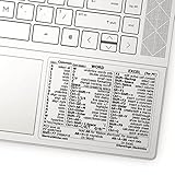
- 💻 ✔️ EVERY ESSENTIAL SHORTCUT - With the SYNERLOGIC Reference Keyboard Shortcut Sticker, you have the most important shortcuts conveniently placed right in front of you. Easily learn new shortcuts and always be able to quickly lookup commands without the need to “Google” it.
- 💻✔️ Work FASTER and SMARTER - Quick tips at your fingertips! This tool makes it easy to learn how to use your computer much faster and makes your workflow increase exponentially. It’s perfect for any age or skill level, students or seniors, at home, or in the office.
- 💻 ✔️ New adhesive – stronger hold. It may leave a light residue when removed, but this wipes off easily with a soft cloth and warm, soapy water. Fewer air bubbles – for the smoothest finish, don’t peel off the entire backing at once. Instead, fold back a small section, line it up, and press gradually as you peel more. The “peel-and-stick-all-at-once” method only works for thin decals, not for stickers like ours.
- 💻 ✔️ Compatible and fits any brand laptop or desktop running Windows 10 or 11 Operating System.
- 💻 ✔️ Original Design and Production by Synerlogic Electronics, San Diego, CA, Boca Raton, FL and Bay City, MI, United States 2020. All rights reserved, any commercial reproduction without permission is punishable by all applicable laws.
Troubleshooting the most common failures
| Symptom | What to check |
|---|---|
| F9 does nothing | Set calculation to Automatic; confirm cells contain RAND or RANDBETWEEN, not fixed values; verify thresholds and the Applies to range. |
| Every light has the same color | Look for a fixed reference such as =$B$2. Use independent formulas or relative references. |
| Icons appear in the wrong cells | Open Conditional Formatting → Manage Rules. Correct the selected range and ensure the formula’s first reference matches its top-left cell. |
| The trunk or star changes color | Rules overlap. Move the trunk/star rule above the light rules, or use Stop If True where appropriate. Rule order determines which format wins. |
| The pattern changes unexpectedly | That is normal for volatile random formulas: opening, editing, or recalculating can produce a new arrangement. |
| The workbook becomes slow | Keep the decorative area small. Volatile formulas and conditional formatting across large unused ranges add calculation work. |
Freeze the pattern or remove the tree
Keep one arrangement
Copy the light cells, then choose Paste Special → Values. The current numbers remain, but the random formulas—and therefore the automatic changes—are removed. Leave the conditional formatting in place if you still want the colors.
Undo the effect
- Select the light range and choose Home → Conditional Formatting → Clear Rules (from selected cells or the whole sheet).
- Delete the decorative cell range if you no longer need the tree.
- Restore gridlines from the View tab.
- If you changed calculation to Manual, return it to Automatic.
Optional upgrades—and their limits
Add presents, a garland, or multiple trees by formatting more cells. A single-cell “refresh” button can be explained to users as “press F9,” but a true unattended flash requires VBA or another repeated-recalculation mechanism. That introduces macro-enabled files, security prompts, performance costs, and compatibility concerns, so the no-macro version is the safer choice for sharing.
The effect works well for a holiday greeting, classroom demonstration, or playful internal dashboard. It is less suitable for a serious operational workbook where volatile formulas and decorative conditional formatting could distract users or affect performance.
Outdated Drivers Are Slowing You Down
One free scan finds every outdated or missing driver and matches the right update for your exact hardware.Free scan · exact hardware matchPC Slower Than It Used to Be?
A free scan shows the junk files, broken settings and background clutter dragging Windows down - then fixes them in one click.Free scan · Windows 10 & 11Quick Recap
Sources and further examples
- Microsoft: Use conditional formatting to highlight information
- Microsoft conditional-formatting example workbook
- How2Excel: Simulate Christmas tree lights
- ExcelIsFun: sparkling tree example
- ExcelIsFun: twinkling tree example

Product prices and availability are accurate as of the date/time indicated and are subject to change. Any price and availability information displayed on Amazon at the time of purchase will apply.